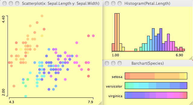
Mondrian is a general purpose statistical data-visualization system. It features outstanding interactive visualization techniques for data of almost any kind, and has particular strengths, compared to other tools, for working with Categorical Data, Geographical Data and LARGE Data.
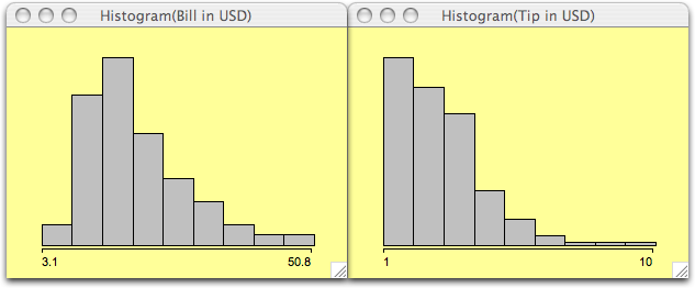
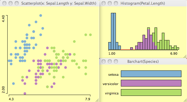
All plots in Mondrian are fully linked, and offer many interactions and queries. Any case selected in a plot in Mondrian is highlighted in all other plots.
Currently implemented plots comprise Histograms, Boxplots y by x, Scatterplots, Barcharts, Mosaicplots, Missing Value Plots, Parallel Coordinates/Boxplots, SPLOMs and Maps.
Mondrian works with data in standard
tab-delimited or comma-separated ASCII files and
can load data from R
workspaces. There is basic support for working
directly on data in Databases (please email for further info).
Mondrian is written in JAVA and is distributed as a
native application (wrapper) for MacOS X and Windows.
Linux users need to start the jar-file. The latest
version can be downloaded here.
If you have any questions or comments, please email mondrian@theusRus.de. Bugs may be submitted to the bug-tracker as well as per email.
News:
- (09/27/22) New versions for
Mac added. There are two separate downloads for Intel
and M1 both including a full JRE. Download is 50MB(!)
now.
- (12/28/21) Updated the note
regarding the Apple
Security setting issue to make Mondrian start
under Mac OS X 12 again.
- (08/29/13) New nightly build version
1.5b, fixing performance problems in very large
maps and previewing the new universal importer.
- (07/31/13) Posted some sample
demo videos created by Antony Unwin. Once we get some more
videos, there will be a video section on this page!
- (10/03/12) Added new maps
for France to the Map
Library
- on departmant level (96 departments), and
- on regional level (22 regions)
- (01/11/11) New release: Version 1.2
The scatterplotsmoother now includes "principle curves", which are one of the nonlinear generalizations of principal components. All smoothers can be plotted for subgroups, which have a color assigned, "smoother by colors".
The color scheme has been refined once again, to make use of colors as efficiently as possible. The use of alpha-transparency is now consistent between scatterplots and parallel coordinate plots.
New Transformations: columnwise minimum and maximum. Sorting of levels is now stable, i.e. levels which have the same value for an ordering criterion will keep their previous order.
The Reference Card speaks Windows now, i.e., Windows users no longer need to translate keyboard shortcuts from the Mac world.
(Filed bugs fixed since last release: 19, 64, 82, 104, 150, 153, 155, 160, 161, 185, 186)
- (01/02/11) The web page has been
reworked and
several issues have been fixed:
- A new section with
a Quickstart Guide
- The order of the plot types now reflects their complexity.
- Technical implementation details are now given where appropriate
- The Map Library has
been opened and we hope for many contributions
- (09/10/09) The slides
which go with the book "Interactive
Graphics for Data Analysis – Principles and Examples"
can now be found on the web.
They should be a fruitful resource for everybody who wants to learn how to use Mondrian.
|
 |
- (05/24/07) we have a
Bugzilla based bug-tracker online. Please submit
all bug reports and requests there - feel free to
email after submission as well ...
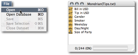
You only need a few clicks to get started using Mondrian:
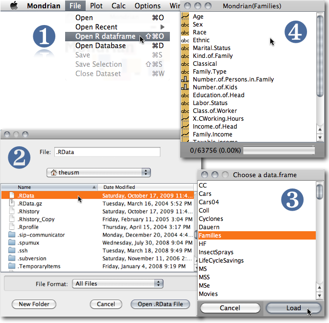
To open a dataset just go to the File menu and choose 'Open':
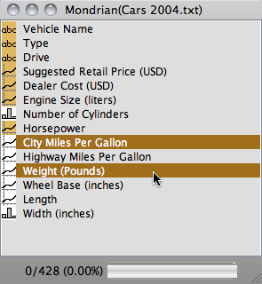
The variable window is the central hub of a Mondrian dataset. Here is what you can read from the window:
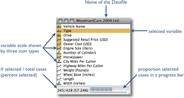
You can find more details in the book "Interactive Graphics for Data Analysis – Principles and Examples", but you should be up-and-running for now.
Also take a look at the sample videos created by Antony Unwin, giving you a nice intro into how you can use Mondrian.
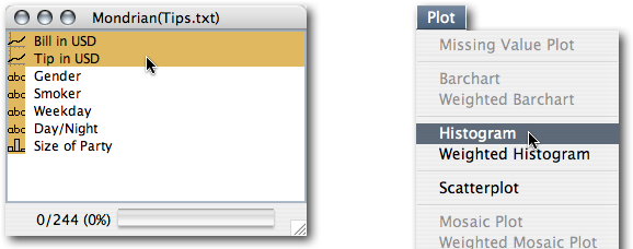
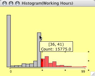
The crucial issues in plotting histograms are to choose the ''right'' number of bins and the ''right'' origin of the first bin. Since there are many rules and hints as to what ''right'' means under different assumptions, the most important interactive manipulations for histograms are changing the number (or width) of the bins and the origin. This is done by pushing the arrow keys (up and down changes the number of bins, and left and right moves the origin). In order to keep the visual distortion as small as possible, the scale of the histogram axis is not updated during the interactive reparametrization. Obviously the y-scale therefore represents probabilities and not counts.
<meta>-0 adjusts the y-scale to the window size after the bin-width has been changed.
The context menu allows you to set a fixed bin width and origin, either by using the suggested "rounded" values or by entering arbitrary values in the dialog box. Furthermore, you may choose from two variations of the histogram, the spinogram and the CD-plot, both showing conditional distributions, which give a good idea of the distribution of a selected subsample.
When Rserve and R are installed, density estimation will enhance the histograms greatly.
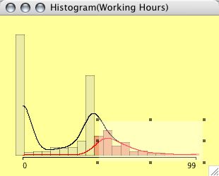
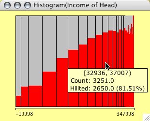
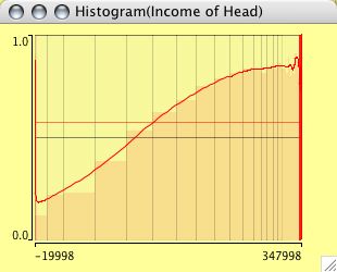
(The right plot shows actually a CD-plot)
Histograms can be weighted. Select two continuous variables (the weights usually should be positive, although Mondrian will not complain about negative weights) and choose weighted Histogram from the plot menu.
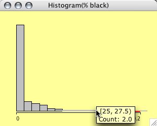
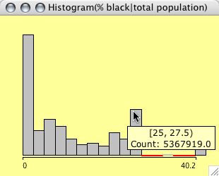
The example shows a typical situation for weighting in a histogram. The left plot shows the distribution of %blacks for the US Midwest counties. The right plot is weighted with the total population, thus showing us the number of people living in areas with a certain % of blacks.
Some technical definitions of histograms:
Default anchor point: Minimum of sample
     Default binsize: (Maximum - Minimum) / 8.9 -> 9 Bins

R-code for density estimation:
> # no weights
> density(x, bw=bWidth, from=Min, to=Max)
> # weights
> density(x, bw=bWidth, weights=w/sum(w, na.rm=T), from=Min, to=Max)

The density estimate for the selected subsample of size SelN is scaled
by a factor SelN/N.

The bandwidth bWidth of density estimators is always identical to the
current binwidth of the histogram itself.
Boxplots y by x are for a single continuous variable, split by a second categorical variable. To invoke a boxplot y by x select the continuous variable to plot and the categorical variable to split by and select 'Boxplot y by x' in the 'Plots' menu.
Manual reordering of the classes is
possible by reordering the levels in a corresponding
barchart.
The context menu offers options to
sort the levels by either median or IQ-range (and to
reverse a current ordering.)
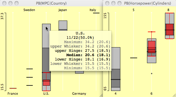
Boxplots y by x for the cars data set
- heavy cars selected.
Parallel boxplots are very similar to
parallel coordinate plots,
and share most of their functionality.
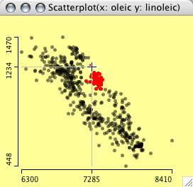
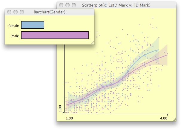
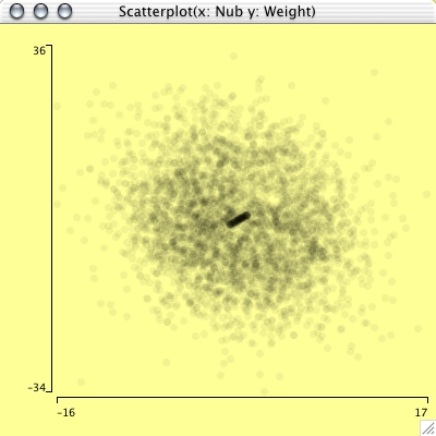
Scatterplots offer all basic interactions: data can be selected and highlighted, the scale can be zoomed.
In contrast to other plots in Mondrian, scatterplots offer axis information, showing the maximum and minimum for orientation.
Query methods for scatterplots operate
on three levels. The first level simply gives the
position of the cursor, which is displayed as a
projection on the x- and y-axes. This query is invoked
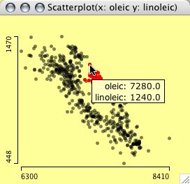
by pressing the alt key. Pressing control invokes
the second level of querying. A tooltip is presented
with the data of the variables in the plot for the
points at the cursor. If more than one point is found at
the same distance, a list of the cases is presented in
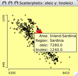
the tool tip. Holding shift and control shows the information of any selected
variables in the variables list, i.e., an extended query
showing data, which are not displayed in the plot.
 |
 |
 |
| orientation | objects | extended |
Three levels of queries in a scatterplot
 |
Example of an image
query which shows a photo of the car, which
turned out to be an outlier in the MDS. In many cases it is very helpful to get additional information for an object, which might only be captured in an image, e.g. a chemical structure or a movie poster. Mondrian allows you to specify a URL for an image location for each case. This can be an entire URL for every case, or a URL composed of a common part and a case specifc part. The common part of the URL is coded in the column name, the case specific part is the entry in the column. |
| The format is as follows: A
column holding image URLs must start with '/U'. If
there is a common part, it follows after the
prefix. The position where the individual entry of
the case goes is enclosed with '<' and '>';
this also defines the column name. Example: |
|
When Rserve and R are installed, scatterplots can be enhanced with scatterplot smoothers. Currently the list of smoothers comprises:
- least square regression (does not need R)
- loess smoother
- regression splines (with confidence intervals)
- principle
curves
There is an option to compare the highlighted smoother either to all data or to the complement.
If colors are defined via color brushing or direct color assignment, smoothers are shown for all colored subgroups.
Defaults and definitions in scatterplots:
Initial pointsize: 3 points (in-/decrease +/- 2 points)
Initial alpha-transparency:

  if( n < 400 )
    alpha = 0%
  else if ( n < 800 )
    alpha = 25%
  else if ( n < 1600 )
    alpha = 50%
  else if ( n < 3200 )
    alpha = 62,5%
  else if ( n < 6400 )
    alpha = 75%
  else
    alpha = 87,5%

Definition of Smoothers
(with "smoother" being a positve integer degree of smoothness, "xf" the
 points where the smoother shall be evaluated.)
>
> # loess
>
> predict(loess(y ~ x, span=3.75/smoother,
                       degree=1,
                       family=symmetric,
                       control = loess.control(iterations=3)),
                       data.frame(x=xf)
         )     )
>
> # splines
>
> predict(lm(y~ns(x, smoother)), interval="confidence", data.frame(x=xf))
>
> # principle curves
>
> principal.curve(as.matrix(cbind(x,y)), spar=0.3+6*(1/smoother+2))
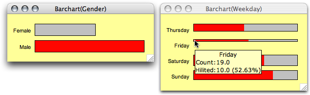
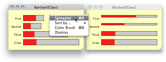
Barcharts in Mondrian follow a vertical layout, not the traditional horizontal layout. Thus the category-names can be printed in full (in most cases).
Besides standard selection and interrogation techniques, interactivity in a barchart includes:
- Reordering of levels via drag &
drop (use <alt>-click on a bar or its text to
drag)
(Dropping between categories inserts, dropping on categories exchanges categories) - Switch between proportional width
and height, between barchar and spineplot
- Sort levels by
- frequency
- name
- absolute highlighting
- relative highlighting
- Reverse current order
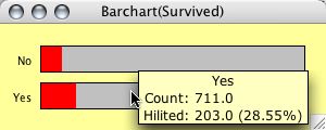
A barchart for the Titanic dataset. First class passenger are highlighted.
(The same behavior can be found in the variables window - plus additional selection of the hits.)
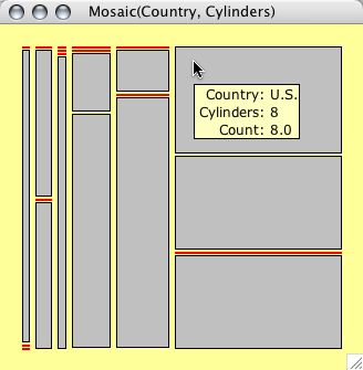
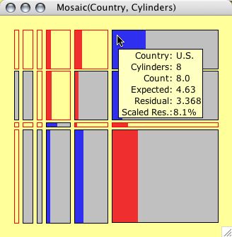
Mosaicplots in Mondrian are fully interactive. Interactivity includes the standard operations described in the convention section (except zooming), plus reordering of the plot variables using the 4 arrow keys. Use <meta>-r to rotate the direction along which the last variable in the plot is split.
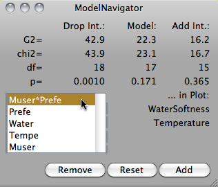
Use <meta>-+ and <meta>-- to add and delete interactions during the modeling process using the ModelNavigator. During the model process one may want to use the plot option to show the expected values of the model and not the observed values.
The picture below shows an example from the Titanic dataset, which includes information on the class (1,2,3 crew), age (child, adult) and gender (male, female) of the passengers. Surviving passengers are highlighted.
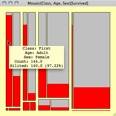
Although there are no labels to decode the cells, the order of the variables is given in the title of the window. Using interactive querying it is easy to check what the cells represent. In this static representation the fact that there are no children and hardly any women in the crew, should be sufficient to decode the plot.
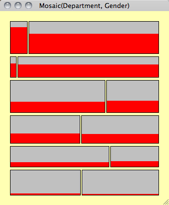
Example of a rotated Mosaic plot, i.e. first variable is split along y not x.
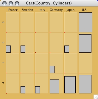
Additionally Mondrian features four
variations of mosaicplots. The figures below show the
same data from the cars data set, in all five possible
variations. Use the pop-up menu for the plot options:
Observed values
Expected values
(according to current model)
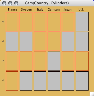
Same bin size
Fluctuation
diagram
These plots show the
five different variations of mosaicplots.
Whereas the first two options are "real"
mosaicplots, the other three versions (same bin
size, fluctuation diagram and multiple barchart)
are more useful for handling only a few
variables with many categories, which is the
worst case for a standard mosaicplot.
For these three variations, Mondrian plots the
category labels for the first two variables,
since the categories are equally spaced and so
can be easily labelled.
By typing shift-up-arrow and shift-down-arrow,
the size of boxes can be zoomed. As soon as a
box reaches its maximum size, it is red-framed
to indicate the incorrect size.
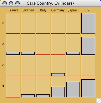
Multiple barcharts
Value Plot
If the dataset has missing values, a missing value plot can be used to analyze the structure of the missing values (monotone missingness etc.).
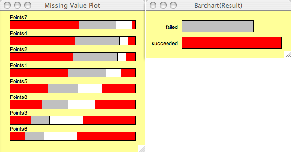
In a missing value plot, only those variables are shown, which actually have missings.
The options of the missing value plot are similar to those of a barchart (sorting etc.)
Missing values MUST BE CODED AS "NA"!!
Coordinate
Plot
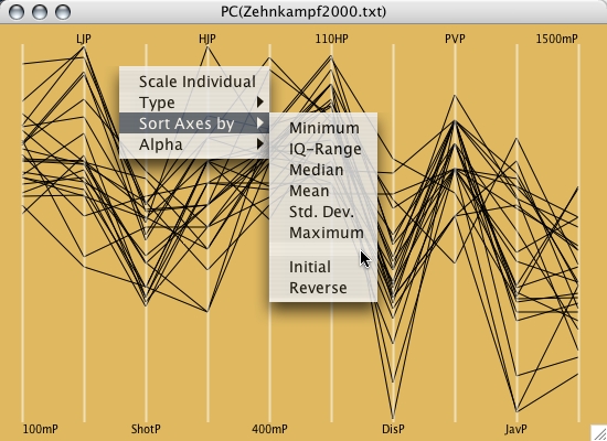
Mondrian implements parallel coordinate plots for an arbitrary number of variables. Alphanumerical categorical variables are displayed equally spaced according to the currently defined order. Numerical variables are scaled according to their actual numbers.
Besides standard selection and querying, interactivity in a parallel coordinate plot includes:
- Reordering of the variables via
drag & drop (use <alt>-drag)
- Switch between common and individual scaling (also for selected subsets of axes)
- Adjust α-level of lines via the context-menu or the left and right arrow keys.
- Select Axes by a single click on the axis name and use:
- BACKSPACE to delete this axis from the plot
- <meta>-I to invert the axis
- Type PAGE-UP or PAGE-DOWN
repeatedly to cycle through the minimum number of
orderings for seeing ALL adjacencies of the variables
in the plot.
(Note: For k variables we need [(k+1)/2] permutations as shown in Ed Wegman's 1991 paper)
- HotSelection only shows the currently selected points in PCPs
- Crop Selection removes the currently selected lines from the PCP. Subsequent crop operations allow you to peel a data set. (only works for lines)
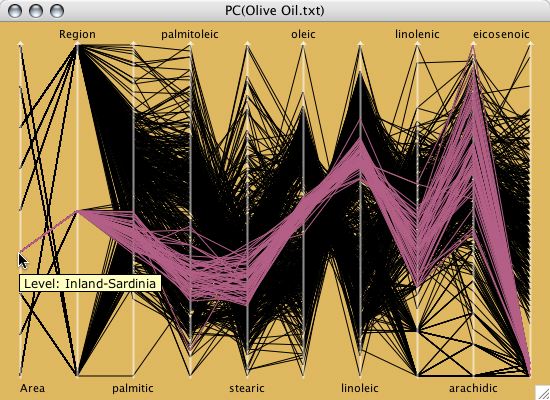
A parallel coordinate plot for the olive oil data.
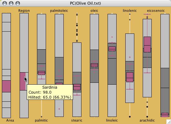
A parallel box plot for the olive oil
data.
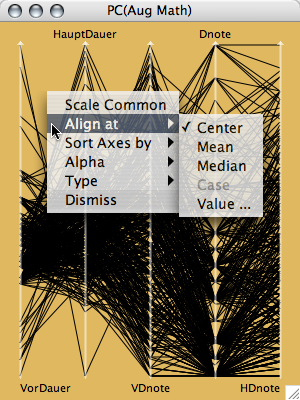
The align menu offers ways to
align/center the axes according to:
|
 |
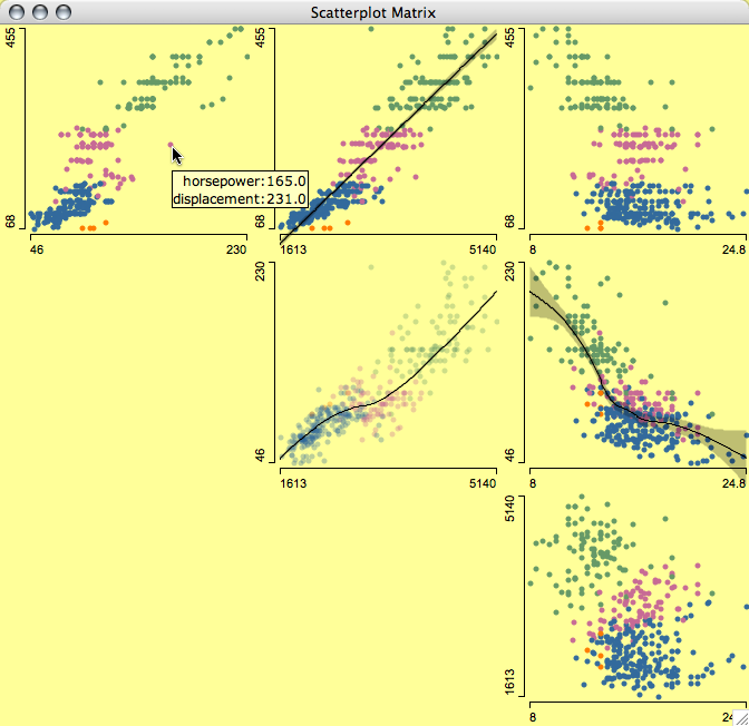
SPLOMs (ScatterPLOtMatrix) in Mondrian are "only" a collection of standard scatterplots, efficiently arranged in a single frame. Thus it has the disadvantage that all keyboard shortcuts apply to all panels simultaneously, but the advantage that each panel is a fully featured scatterplot.
Note:
SPLOMs are quite effective for a quick 2-d overview, but are inefficient when working with more then just a few variables. In the case of many variables, parallel coordinate plots are far more effective.
Whenever a dataset contains information by regions, Mondrian can draw interactive maps if the regions are available as polygons in a separate map file.
A corresponding data record must be provided for each polygon defined in the dataset. Different polygons might point to the same data record, but multiple records to a set of polygons are ignored.
Maps offer the standard selection and querying tools. Additionally the standard zooming function of Mondrian is available.
All maps have a popup-menu at the top
to create a choropleth map of any of the variables.
Further options include:
- Color schemes
- "white to black"
- "red"
- "green"
- "blue"
- "blue to red"
- "blue to white to red"
- if R and Rserve are installed
- "heat"
- "terrain"
- "topo"
- Invert color scheme
- Assign color linearly, normalized, or by rank
- Limit minimum or maximum to a
specific value
 |
 |
| grayscale | green
color scheme |
 |
 |
| blue to red color scheme | normalized
blue to red color scheme |
 |
 |
| normalized blue to white to red scheme | linear
blue to white to red with limit to 30 |
Six choropleth maps of the five Midwest states, shaded according to educational status
The saturation (more precisely the alpha) of boundaries can now be changed with the right arrow key (more saturation) or left arror key (less saturation).
This can change the perception of the map drastically, so make sure to test it out!
US County Map with full saturation:
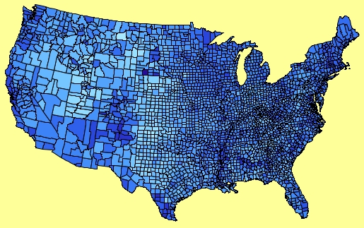
US County Map with reduced boundaries:
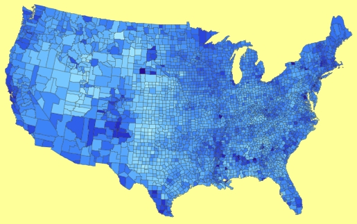
Note the extreme difference between the maps. (We call this technique map-martinizing…)
Color scheme definition in Maps:
Mappings:

- linear
    intensity = (value-min) / (max-min)

- rank
    intensity = rank(value) / n

- normal
    intensity = (qnorm( rank(value) / n )+3)/6;

Color Schemes:

- grayscale
    RBG(1-intensity, 1-intensity, 1-intensity)

- red
    RGB(1-intensity^4/2, 1-intensity, (1-intensity)^3/1.5+0.15)

- green
    RGB( 1-intensity, 1-intensity^4/2, (1-intensity)^3/1.5+0.15)

- blue
    RGB((1-intensity)^3/1.5+0.15, 1-intensity, 1-intensity^4/2)

- blue to red
    RGB(intensity, 0, 1-intensity)

- blue to white to red
    if( intensity < 0.5 )
       RGB(2*intensity, 2*intensity, 1)
    else
       RGB(1, 1-(intensity-0.5)*2, 1-(intensity-0.5)*2)

if R and Rserve are installed

- heat
- terrain      (see R documentation for details)
- topo
Selections in Mondrian can be made in two ways.
- Simple selection
- Selection sequences
Simple selections are performed as any selection in the operating system's desktop. A new selection replaces the current selection.
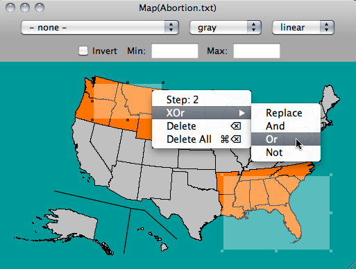
Holding down the <shift> key will combine the new selection with the currently selected data in XOR-mode.
Holding down <shift> and <alt> will perform a selection in extended mode, which is AND by default, but can also be changed to OR in the Options menu.
When using Selection Sequences, any selection is recorded. The selection is represented by a transparent rectangle with 8 handles. Use any of these handles to resize the rectangle (slice) or click-drag the rectangle to move (brush). The popup-context menu on a selection rectangle will indicate the selection step and offer the choice of changing to a different selection mode (union, intersection, negation, xor), of deleting this step, or of deleting the complete sequence. Deleting a single step can also be performed by <backspace>. Use <meta-backspace> to delete the complete sequence. To query objects covered by a selection rectangle hold down the <shift> key to click through the rectangle.
Selection Sequences can span across plots and more than just one selection can be made per plot. To keep track of the selections made, all selections are annotated in the windows menu, just behind the window title, i.e. "Scatterplot(x,y) [2] [4]" tells us that selection steps 2 and 4 have been made in the scatterplot of the variables x and y.
Use <meta>-a to select all cases.
Note: Deleting all selections is not limited to the current plot window.
Brushing
Whereas selections are a more transient technique to mark a subgroup of interest, color brushing persistently assigns colors to cases. There are three ways to define persistent colors in Mondrian
- Definition in a barchart or a
mosaic plot using <meta>-b assigns a discrete
scheme
- Definition in a histogram using <meta>-b assigns a continuous "rainbow"-scheme
- Individual colors may be assigned using <meta>-1 to <meta>-9
 |
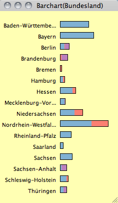 |
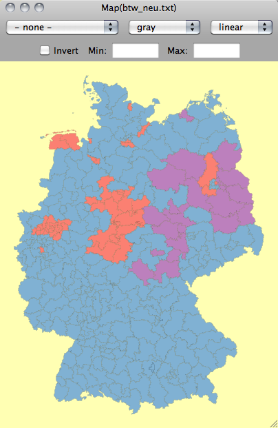
| LEFT: The map of the German electoral districts is colored according to the party winning the most votes in 2009. TOP: The barchart shows the same coloring for the different states. |
To clear all colors use either the (context) menu option or press <alt>-<meta>-b.
Color-brushing is useful, but one should keep in mind two critical issues:
- Permanently defined colors always interfere with the highlighing color and may cause confusion
- Whereas overplotting is no problem for highlighting (highlighted cases are alway plotted on top) the overplotting issue with multiple colors can not be resolved satisfactorily (α-transparency won't work well here).
Qualitative (i.e., discrete colors)

// Color Brewer: 12, qualitative, Set3

   Color[1]  = RGB(128, 177, 211)
   Color[2]  = RGB(188, 128, 189)
   Color[3]  = RGB(179, 222, 105)
   Color[4]  = RGB(253, 180, 98)
   Color[5]  = RGB(252, 205, 229)
   Color[6]  = RGB(141, 211, 199)
   Color[7]  = RGB(251, 128, 114)
   Color[8]  = RGB(204, 235, 197)
   Color[9]  = RGB(255, 237, 111)
   Color[10] = RGB(190, 186, 218)

   Color[11..20] = Color[1..10].darker()
   Color[21..30] = Color[1..10].darker().darker()
   Color[31..  ] = Color[1..10].darker().darker()


Quantitative (i.e., continuous colors)

   for(i=1..k)
     brushColor[i] = HSB(0.225 + i/k*0.8, 0.5, 1.0);
The key to a smooth and efficient user interface is a set of conventions. Once the user has learned the basic operations like selection, querying, zooming and reformatting, she can perform them in any plot.
In an interactive graphical system, possible interactions can be carried out with mouse and keyboard. Since JAVA programs are not bound to a specific platform, Mondrian tries to only makes use of features, which can be found on all platforms. There are some restrictions like the one-button-mouse for most MAC-users (Steve give us the right button!!). The most commonly found modifier keys are SHIFT, CONTROL, ALT and META. CONTROL is blocked as the popup-trigger on the Macintosh, META misused under Windows and ALT blocked by many window-managers under Linux.
The interactions in Mondrian are assigned as follows:
- click -> select a single object
- click and drag -> create a selection (rectangle)
- META-click
and drag -> zoom in/out (middle-click
(wheel) and drag on Windows & Linux)
- CTRL and mouse-over -> query object (use CTRL-SHIFT to get extended query)
- ALT and
mouse-over -> query coordinates in plot
- popup-trigger on background -> alter the plot setting
- ALT-click and drag -> reorder objects
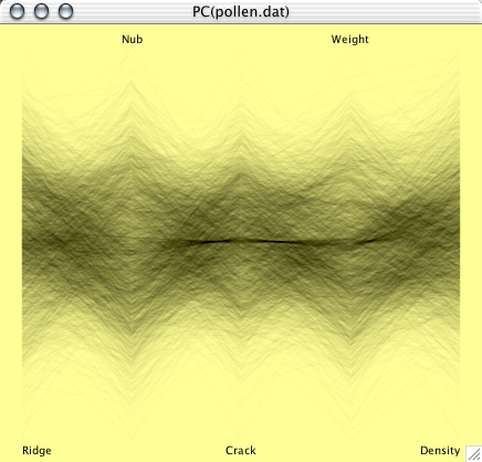
The α-channel can be used to specify the transparency of a painted object. This is very useful, when plotting many objects, as then heavy overplotting can occur. In this way the density of objects can be approximately displayed.
The figures below show an application using the well known "pollen" dataset.
Although Mondrian was not designed to support statistical modeling of datasets, a graphical modeling technique for categorical data using mosaicplots is built in.
The so-called ModelNavigator allows a stepwise graphical modeling of loglinear models.
The ModelNavigator basically inverts the use of graphs and models. Whereas packages like R or S-Plus usually assume a model, for which diagnostic plots can be plotted, the approach in Mondrian starts with a graph, then sets up a model, and uses the statistical measures as diagnostics, to check the graphical conclusions.
For a more precise description of this
technique see the paper on Visualization
of
Loglinear Models.
Mondrian supports the standard ASCII data format, which consists of a header line of variable names and tab-delimited columns.
Numerical and alphanumerical data are both allowed. See example below:
U.S. Buick Estate Wagon 16.9 4.36 155
U.S. Ford Country Squire Wgn 15.5 4.054 142
U.S. Chevy Malibu Wagon 19.2 3.605 125
U.S. Chrysler LeBaron Wagon 18.5 3.94 150
U.S. Chevette 30 2.155 68
Japan Toyota Corona 27.5 2.56 95
Japan Datsun 510 27.2 2.3 97
U.S. Dodge Omni 30.9 2.23 75
Germany Audi 5000 20.3 2.83 103
Sweden Volvo 240 GL 17 3.14 125
Sweden Saab 99 GLE 21.6 2.795 115
France Peugeot 694 SL 16.2 3.41 133
...
The mode of numerical variables can be set interactively:
 |
Double
click
(or use <meta>-T if you need to change more
than one variable) a continuous variable ( ) to change it to be categorical
( ) to change it to be categorical
( ). Vice versa double click to change to . ). Vice versa double click to change to .Alphanumerical variables are tagged as  and cannot be changed to another
type. and cannot be changed to another
type. To get a fast and effective overview of which variables have missings, there are 'white'-versions of the icons of all three types, i.e.  , ,  and and  indicating at least one
missing in the particular variable. indicating at least one
missing in the particular variable.When working with very many variables, just type the prefix of a variable name to search for a particular variable and to make the variable window select all those variables and also scroll to the first hit. |
numCases <- Number of instances in the datasetPolygon Data must be stored in a separate map file.
numCat <- Number of distinct cases in a variables
if( not is.numerical(x) ) then
mode(x) <- "alphanumerical"
else
if ( numCases > 800 ) then
if( numCat < 15 * log( numCases )/log(10) - 1 )
mode(x) <- "categorical"
else
mode(x) <- "continuous"
else
if( numCat < 1.5 * sqrt( numCases )
mode(x) <- "categorical"
else
mode(x) <- "continuous"
The threshold as R code snippet:
>
> i <- 1:1500
>
> plot(i, (i>800)*(15 * log(i)/log(10) - 1) + (i<=800)*(1.5 * sqrt(i)),
type='l')
>
The format for map-data
The dataset must
include one variable of references, which the polygons
refer to. This variable must start with '/P'. If a dataset is asociated with polygons,
there must be an empty line after the data matrix
followed by the relative path+filename to the file
containing the map data.
In the map file,
each polygon must be defined as follows:
It must start with a header like
id \t name \t n
where id is the matching id from the
reference variable. Name can be any arbitrary string
naming the polygon. n is the number of points in the
polygon.
This header is followed by x and y
coordinates defining the polygon - separated by tabs,
one pair per line. The first and last coordinates must
match, i.e. the polygon must be closed.
An example for
Union county:
...
-1.3050 0.7141
1761 /Pnew jersey,union 25
-1.2981 0.7112
-1.2997 0.7100
-1.2995 0.7097
-1.2990 0.7099
-1.2988 0.7098
-1.2991 0.7094
-1.2992 0.7090
-1.2999 0.7086
-1.2985 0.7088
-1.2969 0.7089
-1.2969 0.7088
-1.2964 0.7087
-1.2954 0.7088
-1.2951 0.7090
-1.2947 0.7095
-1.2945 0.7095
-1.2942 0.7100
-1.2942 0.7102
-1.2945 0.7103
-1.2949 0.7103
-1.2956 0.7106
-1.2965 0.7108
-1.2970 0.7107
-1.2976 0.7108
-1.2981 0.7112
1762 /Pnew jersey,warren 33
-1.3112 0.7149
...
Mondrian supports loading data directly from R workspaces. To do so, you only need to specify the R workspace file (in most cases it will default to .RData). Once the workspace file is chosen, Mondrian lists all dataframes within this workspace. Selecting the desired dataframe will dump a temporary file from R and read this file into Mondrian.
The following command is used to dump the data within R
> write.table(rDataSetToDump,
              "<WhereYourWorkspaceSits>/.MondrianTmpImport.txt",
              quote=FALSE,
              sep="\t",
              row.names = FALSE)
Connections
The development version of Mondrian allows the connection to databases via the JDBC interface.
Currently this type of connection, which leaves the data entirely inside the database, is under further development and is thus not available in the latest releases.
The figure below shows the database connection dialog:
There is no doubt, that computations and transformations of data are better done in R than in Mondrian. Nonetheless, there are some basic transformations we want to be able to perform within Mondrian, without being forced to go to R.
The simple transformations include
- +, -, *, /There are also two multivariate transformations which perform dimension reduction
- -x, 1/x
- log(x), exp(x)
- min(x1, ..., xk), max(x1, ..., xk)
(creates two new variables, one with the value,
one with the variable label)
MDS (multidimensional scaling)
creates a scatterplot of the 2-d scaling:
>
> tempD <- dist(scale(tempData))
> is.na(tempD)[tempD==0] <- T
> startConf <- cmdscale(dist(scale(tempData)), k=2)
> sMds <- sammon(tempD, y=startConf, k=2, trace=F)
>

PCA (principal component analysis)
creates k principal components out of k input variables
>
> pca <- predict(princomp("+call+" ,
                          data = tempData,
                          cor = [FALSE|TRUE],
                          na.action = na.exclude))
>
Here are some sample datasets, which are ready to load and test with Mondrian (make sure to save the link directly to preserve the tabs):
Titanic
Olive Oils
Since the new map format was introduced, map files can be used separately from a specific data file. This allows sharing of map-files, such that users don't need to create their own maps, but can build upon the work of others. Here is a first collection of map files:
| Files |
||||
| Area | Level | Map | Data |
Contributor / Remarks |
| World | States | World.map |
World.txt | based
on
the S world map (~ 1998 borders) |
| US | States |
US_States.map | US_States.txt | US States
incl. Akaska and Hawaii |
| Counties |
US_Counties.map | US_Counties.txt | US Counties excl. Akaska and Hawaii | |
| Germany |
States |
Bundeslander.map | Bundeslander.txt | 16 German
federal states |
| Voting
Districts |
Wahlkreise.map | Wahlkreise.txt | German
electoral
districts |
|
| ZIP Level 5 |
PLZ5.map | PLZ5.txt | German ZIP
codes |
|
| City
of Munich |
Munich.map | Munich.txt | Admin.
districts
of Munich |
|
| Italy | Regions | Italy.map |
Italy.txt |
part of the
VDS Tech data on Europe |
| France | Regions | France.map | France.txt | part of the VDS Tech data on Europe |
| Departments | MAP_France1.map | FranceD.txt | thanks to
Antony |
|
| ... |
... |
... |
... |
... |
Please feel free to contribute your maps to share them with other users (make sure you don't violate any copyright and only submit maps that are in the public domain). The data files here are dummies, which connect to the ids in the map file and identify the polygons by region name or region id.
The R-package maptools allows importing MapInfo® files into R and exporting these files in Mondrian format. Here is a short R-code snippet which should basically do the job:
>We hope to grow the map library soon, so many Mondrian users can benefit from using maps in the public domain. There is also a collection of SHP-files at VDS-Technology.
> library(maptools)
>
> # get an example shp-files and unpack it
>
> system("wget http://www.vdstech.com/mapdata/brazil.zip")
> system("unzip brazil.zip")
>
> # load via maptools and dump in Mondrian format
> # Note that you get "brazil.txt" and the mapfile "MAP_brazil.txt"
>
> xx <- readShapePoly("brazil.shp")
> sp2Mondrian(xx, file="brazil.txt")
>
(Everybody who ever used their own data in MapInfo® on a Windows machine will find the map handling and interactive features in Mondrian amazingly fast and flexible)
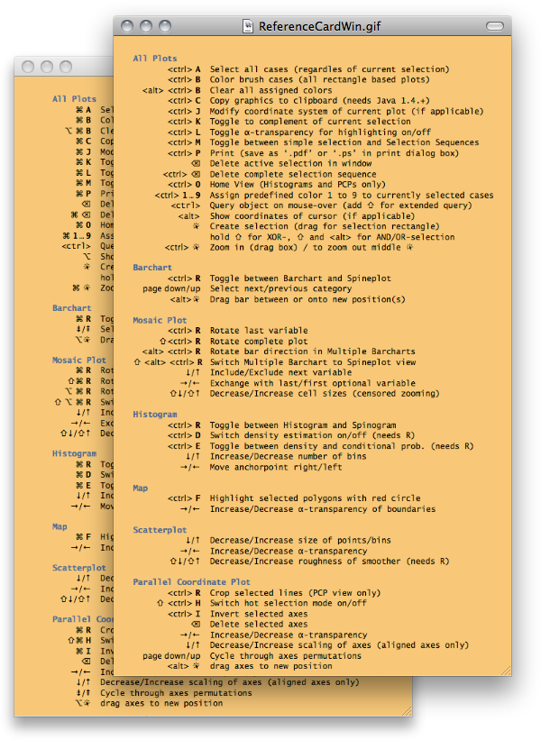
If you need help on Mondrian's short cuts, the "Reference Card" is the place to go. It can be accessed from the "Help" menu.
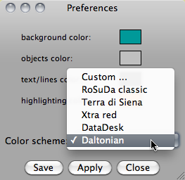
Mondrian features a preferences dialog, to set your favorite background and highlighting color. Five schemes are preset. If you have some other intriguing color scheme, please let me know and I'll add it.
You may save your own customized scheme, if none of the defaults suits you.
Here are the color definitions in RGB HEX

		Background   Objects      Text/Lines   Highlighting
RoSuDa classic	(ff,ff,99)   (c0,c0,c0)   (00,00,00)   (00,ff,00)
Terra di Siena	(df,b8,60)   (c0,c0,c0)   (00,00,00)   (b4,60,87)
Xtra red	(ff,ff,B3)   (c0,c0,c0)   (00,00,00)   (ff,00,00)
DataDesk	(00,00,00)   (00,00,00)   (ff,ff,ff)   (ff,00,00)
Daltonian	(00,99,99)   (c0,c0,c0)   (00,00,00)   (ff,74,00)
By downloading any version of Mondrian, you accept the following license:
Copyright (c) 1997-1998 AT&T Labs Research,
2002-2006 University of Augsburg.
This program is free software; you can redistribute it and/or modify
it under the terms of the GNU General Public License as published by
the Free Software Foundation; either version 3 of the License, or (at
your option) any later version.
This program is distributed in the hope that it will be useful, but
WITHOUT ANY WARRANTY; without even the implied warranty of
MERCHANTABILITY or FITNESS FOR A PARTICULAR PURPOSE. See the GNU
General Public License for more details.
You should have received a copy of the GNU General Public License
along with this program; if not, see <http://www.gnu.org/licenses/>.
Read-only svn-access to the source code:
svn://svn.rforge.net/org/trunk/rosuda/Mondrian/
Binaries for Windows, MacOSX and Linux:
1.5.3 as of 12/31/2021 (still beta)
MacOS (Intel)
MacOS (M1)
(see also note on Apple Security Settings!)
Changes:
- New MacOS versions broke the Java Launcher. JRE is now included in the download!
- Separate Versions for Intel and M1 architecture!
1.5b as of 8/28/2013 (beta version!)
Windows (exe-file)
UNIX (JAR-file)
Mac OS X (Important Note on Apple Security Settings!)
Changes:
Nightly Build Beta including:
- Fixed performance bug in very large maps (>10k polygons)
- First draft of a universal text-file importer
1.2 as of 1/11/2011.
Windows (exe-file)
UNIX (JAR-file)
Mac OS X (Disk-Image containing application and demo data)
Changes:
- Principal Curves
- Smoothers by color
- Further enhancements to color schemes and alpha transparency
- Stable sorting of levels
- Columnwise minimum and maximum transformation
- "Bilingual" Reference Card
- Bug fixes (19, 64, 82, 104, 150, 153, 155, 160, 161, 185, 186) and minor features added
1.1 as of 1/25/2010.
Windows (exe-file)
UNIX (JAR-file)
Mac OS X (Disk-Image containing application and demo data)
Changes:
- Load data directly from R workspace files
- New color schemes
- Compatible with Java 6 on all platforms
- Very many bug fixes (4, 27, 41, 44, 69, 75, 77, 78, 103, 112, 113, 114) and minor features added
Changes in Version 1.0 as of 12/18/2008.
- Autostart of Rserve under Windows and Linux
- Searchable variable list window
- Missing value plot is compatible to color brushing now
Changes in Version 1.0 beta12 as of 08/29/2008.
- Support for Rserve 0.5+
- Fixes and clean-ups
Changes in Version 1.0 beta11 as of 03/19/2008.
- Image can be used in extended queries for URL variables
- New color scheme in maps
- Search in barcharts by typing a prefix of the level
- Fixes and clean-ups
Changes in Version 1.0 beta10 as of 12/16/2007.
- More consistent menu entries and menu labels for plot windows
- A 'Open Recent ...' menu entry
- Indication of missingness in the variable window icons
- Window sizes can now be set in the scale dialog box
- Censored zooming in barcharts (shift up/down-arrow) consistent with mosaic plots
Changes in Version 1.0 beta7 as of 05/13/2007.
- Rserve start-up compatible with Rserve for R2.5.x
- SPLOMs are available now (for those who like'm ...)
- histograms are more consistent now (weighted histograms support densities (needs Rserve), spinograms now work at any zoom level)
- better scaling and queries in parallel boxplots (still incomplete)
- several fixes and enhancements ...
Changes in Version 1.0 beta3 as of 10/31/2006.
- simple transformations (+, *, -, /, log, 1/x, ...)
- selection order of variables in variable window is reflected in all multivariate plots!
- many minor fixes and enhancements ...
Changes in Version 1.0 beta1 as of 05/24/2006.
- new much faster loader (note: maps are now expected to be in a separate file)
- missing values (coded as "NA") are supported in all graphics
- missing value plot can be used to investigate the structure of the missing values.
- custom scaling (<meta>-j), scatterplot only, other plots to follow
- color brushing (<meta>-b) in barcharts, mosaic plots and histograms (rainbow)
- <meta>-1...9 sets persistent colors for the current selection
- derived variables from selection- and color-state
- painting, via "OR"-mode in the first selection step of a selection sequence
- many minor fixes and enhancements ...
Changes in Version RC 1.0m as of 11/29/2005.
- Using 1.4.x JVM on all platforms.
- '<-' and '->' can be used to change the saturation of boundaries in maps.
- "Boxplot y by x" is now a separate menu item.
- Levels can now be sorted in boxplots y by x according to median or IQ-range.
- Plotting of 2-dim MDS (input is not carefully checked yet)
Changes in Version RC 1.0f as of 04/06/2005.
- Queries are now implemented via ToolTips.
- Further improvements to Parallel Coordinate Plots. See section for details!
- Maps now feature six different color schemes for shading choropleth maps.
- Under MacOSX you can now drop files on Mondrian to start the application and load the data.
- If you have R and Simon's Rserve installed on your machine, you find new features in
+ Histograms
+ Scatterplots
Changes in Version RC 1.0 as pf 09/24/2004:
- Vast improvements to Parallel Coordinate Plots. Se section for details!
- Printing works via <meta>-P in all plots. In MacOS X use "Preview" to save as PDF.
- Additional sorting options in Barcharts.
- Histogram parameters can now be set manually as well.
- Choropleth maps can now be inverted and colored by rank.
- Yet another update to the L&F of selection sequences.
Changes in Version 0.99a as of 03/11/2004:
- an updated version of selection sequences. See the section for details.
- "window" menu and more intelligent window placement
- new controls to set width and origins in histograms
- zooming for all platforms (use middle mouse button on all other machines than mac)
Changes in Version 0.99 as of
11/18/2003
- Three new variations of Mosaic
plots (same bin size, fluctuation diagram and multiple
barcharts)
- Automatic sorting of axes in a
parallel coordinate plot
- Use meta-R to switch the splitting
direction of the last variable in a Mosaic plots
- Inverse color scheme for density
highlighting in scatterplots
- Preference box to set highlight
color and background color
- Zooming under Windows is still
delayed because of a yet to be finalized major update
on the interface
Changes in
Version 0.98 as of 03/22/2003:
- Boxplots y by x. Just select a
continuous variable and a categorical variable and
choose 'parallel boxplots' in the plot menu.
- Regression lines in scatterplots
(can be queried)
- Highlight color is now red!
- Add lines in scatterplots by
third variables to visualize paths and other
relationships.
Changes in Version 0.97a as of 11/21/2002:
- oneClick selection is
introduced, i.e. a selection rectangle of size 0
will only select the clicked object, but NOT
create a corresponding selection rectangle
(selection is only temporary as with the select
all feature (META-a))
- Bug fix in Scatterplots
- Update on selection rectangle
appearance
Changes in Version 0.97 as of
7/12/2002:
- META-a will select all points in any plot now
- alpha-channel works in scatterplots (use arrow
keys to change) and parallel coordinates (via
pop-up).
- scatterplot are automatically binned, if the
dataset is really large (can be overridden)
- interrogation in maps added
First public
release 0.96 as of 4/9/2002
Note: The JAR-file can be started by a simple
double click. Within Windows, Sun's JRE or JDK
must be installed (make sure that .jar files are
not associated with any decompression
application), Mac OS X users just smile.
The best reference for citing Mondrian - apart from the website - is 'the book'.
@book{1502124,
author = {Theus,, Martin and Urbanek,, Simon},
title = {Interactive Graphics for Data Analysis: Principles and Examples (Computer Science and Data Analysis)},
year = {2008},
isbn = {1584885947, 9781584885948},
publisher = {Chapman \& Hall/CRC},
}
There is also the JSS-Paper:
@article{Theus:2002:JSSOBK:v07i11,
author = "Martin Theus",
title = "Interactive Data Visualization using Mondrian",
journal = "Journal of Statistical Software",
volume = "7",
number = "11",
pages = "1--9",
day = "22",
month = "11",
year = "2002",
CODEN = "JSSOBK",
ISSN = "1548-7660",
bibdate = "2002-11-22",
URL = "http://www.jstatsoft.org/v07/i11",
accepted = "2002-11-22",
acknowledgement = "",
keywords = "",
submitted = "2002-07-11",
}
Getting around Apple's security settings
The latest MacOS X versions are quite strict on starting applications downloaded from the web. Changing the security setting in the preference no longer can solve the error which is displayed, when you try to start Mondrian:

Once you copied Mondrian to your Applications folder you may simply fix this problem by opening Terminal and typing:
> xattr -d com.apple.quarantine /Applications/Mondrian.appThis takes Mondrian out of quarantine (an awkward naming choice in COVID-19 times!), where all downloaded apps end up, if they do not adhere to Apple's certificates.
Starting Rserve
Getting a tiny warning message after starting Mondrian only indicates that there is no connection to R. This will NOT harm Mondrian in its core functionality - one can happily live without the R connection.
Rserve is now a regular R package and can be installed as such, i.e. you just need to type the following R command:
> install.packages("Rserve")
Since version 1.0,
Mondrian will start Rserve automatically under MacOSX,
Windows and Linux. To start Rserve manually, see
detailed instructions here.If the automatic start of Rserve fails you may debug within R by typing
> Rserve()to start it manually. Sometimes you may get in trouble with an "old" Rserve server still running after an update of R and/or Rserve. The easiest way to solve this problem is a simple restart.
File Formats
If you have trouble getting data loaded into Mondrian, load the file into MS Excel first, and check whether
- all
variables have a name in the header, i.e. the
first row/line
(When saving data from R without omitting the row names, the "row.name" column has no header name!)
- there
are empty cells in the file. Mondrian
currently does not tolerate empty entries, you
have to use "NA".
If your dataset is more complex or too large, you may do the similar "data cleaning" procedure using R. It is easiest when you use the JGR GUI, which has an "Open Dataset" menu item and allows you to save the file from the object browser.
If you have your data in R already, you may use the "Open R data.frame" command from the Mondrian file-menu.
Starting a JAR File under Windows (if one can't use "Mondrian.exe" for some reason)
After an installation of SUNs latest JRE (or JDK), .jar-files can be started by a simple double click. If this does not work, one of the following two problems might be the cause
- There is no application associated with the suffix .jar. To change this, follow these instructions.
- Another application "grabbed" the responsibility for .jar-files - usually "WinRAR" - after the installation of the JRE. To change this, you must:
- Launch
the WinRAR application
(Start -> Programs -> WinRAR -> WinRAR) - Once the application has been started, select "Options", "Settings".
- Select the "Integration" tab.
- This tab lists all associated file types for the WinRAR application. De-select the "JAR" type and click "Ok".
- Close the WinRAR application.
Other Problems
Please mail to either mondrian@theusRus.de or the mailing list stats-rosuda-devel, or submit your issue to the Bugzilla based bug-tracker.
Topics of general interest will be posted on this page.